On September 10, India’s case fatality rate from Covid-19 stood at an impressively low figure of 1.7%. This is far lower than the world average. The Indian government has not been slow to tout this as proof that India is coping resiliently and well with the pandemic.
The reaction from other quarters has been just as quick but not as positive: India has a particularly young population, which would tend to bring down the fatality rate. The lag between infection and death, coupled with increased testing, could also bring down the fatality rate by expanding the denominator (positive cases) relative to the numerator (fatalities). And of course, there could be severe undercounting of Covid-19 deaths.
In this day and age, with echo chambers cranked up to maximum volume, it is easy to imagine these as largely academic arguments. But of course they’re not. The quantitative effect of these various propositions has implications for the assessment of both intrinsic and comparative performance of countries in combating the pandemic. That said, the emphasized phrase in the previous sentence is important. We need to know how strong these effects are, over and above the mere assertion that these are possible effects.
In Philip, Ray and Subramanian [linked here], we do just this for two of the three counterarguments listed above. We give precise quantitative expression to the relevance of the age distribution, and to the relevance of the lag between infection and death. In this article, we describe our approach, and provide some updated results.
Younger populations
We first describe the two effects of interest in slightly greater detail. First, case fatality rate does not take account of the precise age-specific distribution of Covid cases and Covid deaths. It is well known that younger countries will exhibit lower CFRs simply because the young are more resilient to the virus. In principle, it is possible for a country like India to have a higher age-specific mortality rate, while still enjoying lower mortality on the whole.
Second, there is a time lag that occurs between the onset of infection and the date of death (when infection leads to death, that is). Verity et al [linked here] report a mean (average) duration of around 18 days from infection to death, while Wilson et al [linked here] conclude that “. . . a median of 13 days passed from pneumonia confirmation to death . . . ”.
That suggests that the contemporaneous CFR – deaths on a given date divided by the number of cases at that same date – might be an inaccurate reflection of the true case-mortality rate. We would need to divide by the number of Covid cases at some relevant anterior date; call this the lagged CFR. It is, of course, no surprise to learn that lagged CFR for India is higher; see Mohanty et al [linked here]. But that would be true for all countries in the growing phase of the disease or as testing expands, not just India.

What is more interesting are comparisons across countries, for it is only then that we can note the relative deflation in case fatality brought on by the growth in reported cases. In particular, it is easy to see (and risky to miss) the fact that all else equal, a country with a faster growth rate of confirmed cases exhibits a higher ratio of lagged CFR to contemporaneous CFR.
In what follows, then, we expand on these qualitative observations to get some hard numbers. We ask first: what would happen to India’s CFR if age-specific mortality rates were similar to those in other countries, including older countries? That is, what would predictions for India’s CFR look like, using age-specific fatality rates from comparison countries coupled with India’s distribution of Covid-19 cases? If these predictions are lower than India’s actual performance, it would lend serious credence to the age distribution counterargument. And of course, we could do this for both contemporaneous and lagged CFRs.
A second route to understanding age distribution is via the technique of ‘decomposition’. This is a sharper method, but more demanding on data requirements relative to the prediction exercise, as we need information on age-specific incidence and mortality for both India and the comparison country. One could then decompose the difference in CFRs, and thereby isolate two factors that combine to generate an overall statistic: one corresponding to the difference in CFRs based on differences in case distribution (an ‘incidence effect’), and the other to the difference in CFRs based on differences in age-specific fatality rates (the ‘fatality effect’).
Like the prediction exercise, the decomposition method can also accommodate lagged CFRs with ease. And it is entirely possible that two countries have similar CFRs as a serendipitous consequence of the incidence and fatality effects operating in opposite directions and largely cancelling each other out. The CFR would then generate similar end-state descriptions while concealing vastly differing underlying processes leading up to that end state, a feature shared with many other similarly doubtful summary statistics.
In implementing these exercises, we compare India to a set of 17 other countries for which age-distribution information is either available or can be constructed. Each prediction and decomposition exercise comes in three variants: one with contemporaneous CFRS, and two more with lagged CFRs that employ 14- and 21-day lags.
The decomposition procedure we use is the Shorrocks-Shapley exact decomposition procedure; the outcome of this decomposition coincides with a procedure advanced by Kitagawa (1955) for use in specifically demographic contexts. We are certainly not the first to carry out such decomposition exercises – for similar efforts, the reader is referred to Dudel et al. (2020), among others. The precise arithmetic of decomposition is dealt with in our paper, and is beyond the scope of this article.
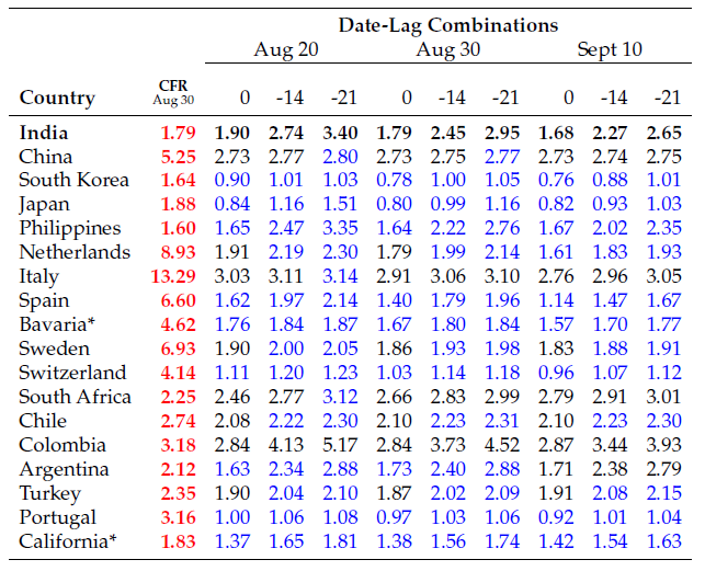
The results of our empirical exercises are summarised in Tables 1 and Table 2. Table 1 contains the prediction exercise. The very first row contains the Indian CFR, contemporaneous and lagged, at three dates: August 20, August 30 and September 10. The rows below contain the corresponding predictions for India that arise from a set of 17 comparison countries.
Let’s take one of them; say Spain. Spain had an average CFR of 6.6% on August 30, over three and a half times as high as India. But the numbers in blue along Spain’s row reveal the hypothetical CFRs (both contemporaneous and lagged) that would have resulted were Spain to have India’s age distribution. Of course, those numbers are lower than 6% – Spain is an older country.
But it’s more than that: the numbers are lower than India’s rates, a much stronger statement. On September 10, Spain’s contemporaneous prediction for India was just 68% of the Indian number. The corresponding prediction for South Korea was 45%. Lagged (by either 14 or 21 days), the predictions fall even more: to about 64% of the Indian number for Spain, and to under 40% for South Korea. These numbers speak for themselves.
More generally, all the underpredictions are highlighted in blue. Alas for India, these are the vast majority of the numbers.

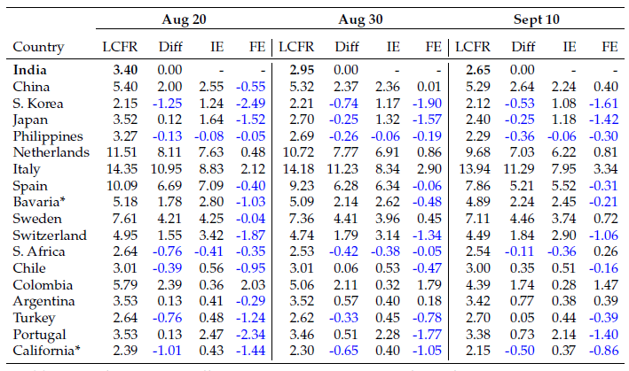
Table 2 summarises the decomposition exercise for a 21-day lagged CFR. India’s rates for three dates are shown on the top row, as before. Now, for any of the comparison countries, and for each of the three dates, the corresponding row lists, first, the lagged CFR, the raw difference with India (“Diff”), the incidence effect (“IE”), and the fatality effect (“FE”). Not surprisingly, the raw differences are generally positive – which is the reason that the Indian government has declared satisfaction with India’s response to Covid-19.
The next column, again generally positive, shows that the bulk of the raw difference is accounted for by the incidence effect in favor of India – the fact that the Indian age distribution is skewed in favor of the young.
The last and most interesting column is the fatality effect. It is related to the prediction exercise in Table 1, but is not quite the same, as it estimates the difference using an average of the Indian and comparison age distributions – the prediction effect uses only the Indian age distribution. In line with the prediction effect, the majority of these terms – highlighted in blue – are negative, suggesting that age-adjusted, India is not doing as well as we might think. In fact, it is safe to say that compared to these 17 countries, India has been performing quite poorly.

As an example of how aggregates could hide patterns, consider Japan on August 30. It had a lagged CFR of 3.5%, just a shade higher than India’s number of 3.4% recorded on the same date. But the incidence and fatality effects are both large, each of these differences accounting for close to half the baseline death rates. The incidence effect works in India’s favor – Japan has the older population. But the fatality effect wipes out this advantage almost entirely: what India has in youth, it gives up in age-specific death rates.
Recall that there are other factors that could perhaps explain India’s low CFR, including the possibility of dramatic undercounting of Covid-19 deaths. After viewing these tables, the reader must judge the extent to which the undercounting of deaths is even needed to explain India’s exceptional numbers.
Undercounting may well be present. We have little to say directly about this possibility, as we do not have the data. But Tables 1and 2 together suggest that an undercounting argument need not even be invoked to understand the large discrepancies. India’s Covid-19 experience does not indicate unqualified success, relative to several comparison countries, with or without undercounting. And at the very least, there is reason to believe that an undiscriminating employment of the raw CFR as an indicator of success deserves to be treated with some scepticism.
It seems to be important to assert this when both objective appraisal and fair accountability are threatened by summary indicators of performance that are inadequate or misleading, and when such summary measures are employed to their advantage by politicians and policy-makers.
Minu Philip is a doctoral student in Economics at New York University.
Debraj Ray is Julius Silver Professor in the Faculty of Arts and Science, and Professor of Economics, New York University.
S. Subramanian, who lives and works in Chennai, is a former professor of the Madras Institute of Development Studies.
This article has been published in collaboration with Ideas for India.


